Content:

1. Thermodynamics

2. Kinetics

_

Thermodynamics

Chemical reactions

Chemical reactions are processes in which one set of chemicals, reactants, change into another set, products. Such reactions are usually described using chemical equations such as (1):

aA + bB → cC + dD

A and B are the reactants, C and D are the products of the reaction. Small letters a, b, c, and d denote stoichiometric coefficients of the reaction, which tell us about the mass ratios of chemical entities involved in the process. The term ‘equation’ suggests an equality between the two sides: in any chemical reaction mass, energy and electric charge must be conserved.

Let us now consider a reaction between cuprous and ferric ions in solution (2):

Cu⁺ + Fe³⁺ ↔ Cu²⁺ + Fe²⁺

Similar to most reactions in chemistry (and almost all in biochemistry) this reaction is reversible, which means that it can proceed in either direction. As such, it will stop at a point when a certain

amount of iron has been reduced and certain amount of copper oxidised. At this point we consider the system to be at equilibrium, i.e. there is no net change of reactants into products or vice versa.

This equilibrium can be mathematically described using an equilibrium constant, K_eq, which is defined as the ratio of equilibrium concentrations of products to those of reactants (to the power of appropriate stoichiometric coefficients). The equilibrium constant for (1) would thus be as follows (3):

K = [C]^c[D]^d / [A]^a[B]^b

and for reaction (2) is (4):

K = [Cu²⁺][Fe²⁺] / [Cu⁺][Fe³⁺]

Let’s assume that the equilibrium constant for reaction (1) is equal to 1, i.e. at equilibrium the products of the concentrations of products and reactants are equal. If we add more compound A into this system, the equilibrium will be disturbed and the chemical reaction restarts in the direction that promises to restore the equilibrium. In this case, A will react with B to form C and D until, once again, the two products of concentrations ([A][B] and [C][D]) are equal and a new equilibrium state is reached.This qualitative rule is called Le Chatelier’s Principle

Chemical potential

We can now ask what makes a chemical reaction move in one or the other direction in response to changes in the chemical composition of the system? One way of putting it would be using an analogy with a seesaw. A fat person sitting on a seesaw with a small person on the other side will very likely move downwards; if there are two people of the same weight on the seesaw, they will eventually end up level.

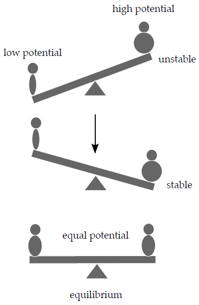
This can be explained by the potential energy of the two people in Earth’s gravitational field. Gravitational potential energy depends on the weight and position in the gravitational field. The system in this analogy, i.e. the seesaw, will tend to minimise its potential energy by moving the fatter person as low as possible. Similarly, we can define chemical potential (μ) as the potential energy stored in a certain amount of a compound, which can be released during a chemical reaction. In an analogous way to our seesaw example in a chemical reaction we have chemicals of differing potentials on the two sides of the equation. If the sum of chemical potentials of the reactants exceeds that of the products the reaction will flow in the direction of the products – and vice versa. If the potentials are equal the system is at an equilibrium.

Gibbs energy

The difference in chemical potentials between products and reactants gives us a new parameter called change in Gibbs energy (ΔG). Gibbs energy has many definitions but two are especially important for biochemistry:

1) Change in Gibbs energy is equal to the maximum amount of (non-volume) work that can be done by the reaction

2) Change in Gibbs energy is a measure of displacement from equilibrium.

The first definition tells us that ΔG can be used to determine whether or not a reaction will occur and whether it can be used to power some other process (muscle contraction, pumping ions across a membrane). The second definition expresses two facts:

1) At equilibrium ΔG is zero

2) Changing the concentration of chemicals in a system away from an equilibrium state will change (increase or decrease) ΔG.

The meaning of Gibbs energy can be also illustrated in a graphical form.

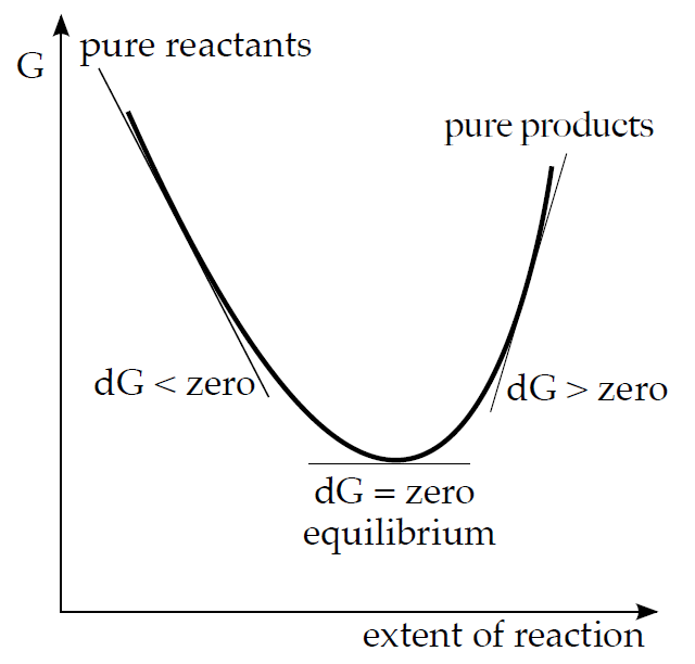
If we start off with a mixture of reactants the reaction will move towards products as long as ΔG is negative. When the chemical potential of products reaches the same value as that of reactants the reaction system reaches a state minimum energy and the reaction stops. The reaction mixture is at equilibrium. The reaction is unlikely to proceed any further since ΔG in that part of the curve is positive.

The change in Gibbs energy can also be defined using other thermodynamic quantities. e.g. enthalpy (H) and entropy (S) (5):

ΔG = ΔH – TΔS

ΔG < 0 spontaneous reaction

ΔG = 0 equilibrium

ΔG > 0 no reaction

Enthalpy is the energy released or consumed during the reaction (negative sign means released enthalpy) and entropy is the disorder of the system. According to the 2nd law of thermodynamics all closed systems become increasingly disordered.

As we can see in (5), chemical reactions can be driven (i.e. achieve negative ΔG) by either favourable (also negative) enthalpy change, or a sufficient increase in entropy or both.

For practical reasons it is useful to define standard chemical conditions, measure DG and other quantities under these conditions and use them to calculate real life situations. In chemistry, standard conditions are 1 atm pressure (101 325 Pa), 25C (298.15 K) and 1 molar concentrations of chemicals. Quantities measured under such conditions are denoted by the superscript ⁰. Biochemists, not to be outdone, defined their own standard conditions with pH = 7 (unlike pH = 0 in the chemists’ version). Biochemical standard quantities can be recognised by having ‘.

From tabulated values for ΔG⁰ or ΔG⁰’ we can calculate DG for any reaction using equation (6):

ΔG = ΔG⁰ + RT ln ([C]^c[D]^d / [A]^a[B]^b)

At equilibrium ΔG is zero and [C]^c[D]^d / [A]^a[B]^b is equal to K_eq. Equation (6) then becomes (7):

ΔG = – RT ln K_eq

This expression allows the calculation of the equilibrium constant from ΔG or vice versa.

The ready availability of ΔG⁰ values brings about one major temptation to all followers of the noble biochemical path. Many a disciple will peruse the tables and upon seeing a positive value of ΔG⁰ will exclaim:“This reaction shall not occur!” Such hastiness, however, would not serve well the novice biochemist.

Let’s look at a real life example. One major metabolic pathway called glycolysis contains a step, in which glucose-6-phosphate is changed into its isomer fructose-6-phosphate. ΔG⁰‘ for this reaction is +1.7 kJ/mol. Does that mean that our cells constantly violate laws of thermodynamics by performing this reaction every second of our lives?

It is essential to keep in mind the difference between ΔG and ΔG⁰ or ΔG⁰‘. Only ΔG tells us something about the thermodynamic profile of a specific reaction. ΔG⁰ and ΔG⁰‘ are only valid if reactants occur in standard concentrations and conditions, which is rarely, if ever, true in nature. In order to evaluate the likelihood of a reaction occurring we must know the real concentrations of all chemicals taking part in the reaction. Since in our cells enzymes continually remove fructose-6-phosphate and thus keep its concentration very low, the overall DG for the isomerisation of G-6-P to F-6-P is negative (-2.5 kJ/mol). This is how some relatively unfavourable reactions can be coupled with more favourable reactions. If reaction A → B tends to reach equilibrium with very low concentration of B (i.e. it runs very poorly) we can link it to a subsequent reaction B → C which, on the other hand, only reaches equilibrium when almost no B is left. The second reaction thus efficiently removes any B formed by the first reaction and prevents it from reaching equilibrium. In our glycolytic example the enzyme phosphofructokinase very efficiently phosphorylates F-6-P to fructose-1,6-bisphosphate and prevents any build-up of F-6-P, which would hinder the proceeding reaction.

Electrochemical equilibria

Chemical reactions involving changes in oxidation number of elements are called redox reactions. Oxidation increases the oxidation number while reduction decreases it. These changes usually involve a transfer of electrons from one atom or molecule to another. Historically, the first redox systems studied were chemical reactions generating electricity.

If we dip a zinc bar into a solution of zinc sulphate a reaction will start in which metal zinc will give up two electrons and change into Zn²⁺ ions until equilibrium is reached. This leads to a build-up of electric charge called electrode potential (E). This potential cannot be measured directly but only as a difference from another potential. Potential difference is what we all know as voltage measured in volts. To overcome the problem with measuring absolute potentials ingenious chemists devised a neat trick: they picked one electrode and assigned to it zero potential. This electrode is called standard hydrogen electrode (she). As a result, E is in fact potential difference sometimes also denoted as ΔE.

Obviously, the amount of electric charge and therefore the value of electrode potential will be related to the equilibrium constant of the reaction. But how? Let’s recall that ΔG is equal to the maximum amount of work that a system can perform. In an electric field work is performed by moving a charge over a potential difference (similar to mechanical work by moving a mass in a gravitational field – like climbing stairs). The relationship between ΔG and E is then (8):

ΔG = – nFE

n is number of electrons transferred in the redox reaction; F is Faraday’s constant (equal to the charge of 1 mol of electrons, approximately 9.6485309 x 10⁴ C.mol^-1)

For standard electrode potential we can write (9):

ΔE⁰ = (RT / nF) lnK

Under non-standard conditions equation (9) becomes (10)

E = E⁰ – (RT / nF) ln [reduced]/[oxidised]

and is called the Nernst equation.

How does one use these equations to calculate whether or not a specific redox reaction is likely to occur? The decisive parameter is, as before, the value of ΔG for the reaction. This can be calculated from equation (8), where E is the overall potential difference between the two half reactions.

Let’s consider a redox reaction like this (11):

Zn + Cu²⁺ ↔ Zn²⁺ + Cu

The two half-reactions are (12) and (13):

Zn ↔ Zn²⁺ + 2e^–

Cu²⁺ + 2e^– ↔ Cu

Zinc is oxidised and copper reduced. Standard electrode potentials are usually tabulated as reductions so the value of E⁰ for the oxidation of zinc will have to be multiplied by -1. The two half-potentials are then added together to give the overall potential of the reaction. In this case E⁰_Zn/Zn2+ = +0.76 V (note the reversed sign due to reversed reaction) and E⁰_Cu2+/Cu = +0.34 V giving the overall potential difference at +1.1V. For reaction (11) under standard conditions the overall potential difference is positive, which means that ΔG (in this case equal to ΔG⁰) is negative and the reaction will spontaneously proceed. Under nonstandard conditions the full Nernst equation must be used for both half-reactions.

_

Kinetics

While thermodynamic analysis answers the question whether a reaction is thermodynamically favourable chemical kinetics can provide the next piece of the puzzle, i.e. how fast and if at all will such a favourable a reaction run in real life.

There are many thermodynamically favourable reactions that do not spontaneously occur. Everybody knows that burning wood in air releases a fair amount of energy which can be used to do work, e.g. in a steam engine. Clearly, oxidation of cellulose and certain polyphenols in pine logs by oxygen to water and carbon dioxide must have negative ΔG. How is it, then, that we can admire mighty pine forests standing in our oxygen-rich atmosphere for centuries? Shouldn’t they have burnt to the ground in an instant?

Similarly, diamonds, which the marketing machinery depicts as ‘being forever’ are but a thermodynamically unstable (i.e. unfavourable) modification of graphite or soot. Under normal conditions they do seem to last a while but if ‘forever’ is what your fiancée wants graphite is a better bet (soot is a little tricky to attach securely onto a gold ring). Buy her a pencil instead!

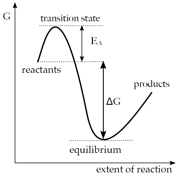
Some reactions may be thermodynamically favourable but kinetically unlikely. Usually the reason for this phenomenon called kinetic barrier is the existence of an unstable intermediate state (transition state or activated complex), which only forms if more energy is supplied (i.e. formation of the intermediate is thermodynamically unfavourable). This additional energy is called activation energy (E_A).

Reaction rate

In order for two or more chemicals to react together their molecules must collide. Such collisions become more likely with increasing temperature, pressure and concentration.

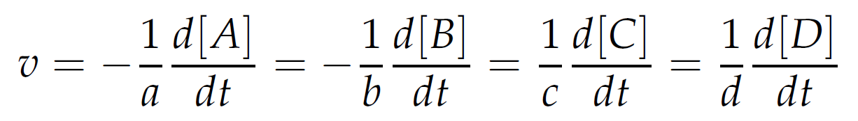
We can define reaction rate (v) as the rate of disappearance of reactants or rate of accumulation of products (14):

How is reaction rate related to the concentration of reactant(s)? Let’s consider a simple reaction X → Y. The rate of this reaction may be proportional to [X] like so (15):

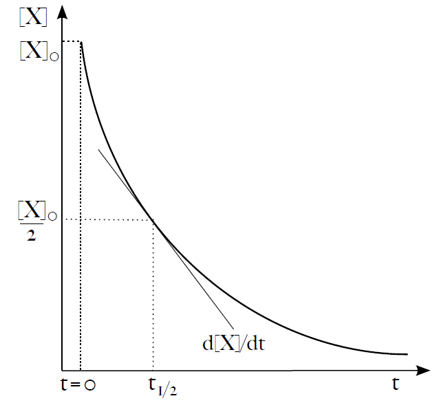
v = – d[X] / dt = k[X]

where k is the rate constant. However, the rate could also be proportional to [X]² or not be proportional to [X] at all – in such a case the reaction proceeds at a constant rate. The precise relationship between reaction rate and the concentration of reactants is an empirical fact and cannot be guessed from stoichiometry. Chemists define kinetic order of a reaction based on the number of entities, whose concentrations affect its rate. If there is no relationship and v = k it is a zeroth order reaction. If the rate is proportional to the concentration of one reactant we call it a first order reaction, e.g. equation (15). If the rate is determined by the concentration of two reactants or one reactant squared (v = k[X][Y] or v = k[X]²) it is a second order reaction. And so forth.

Sometimes we would like to predict how much reactant X will be left after time t or how long it will take for [X] to fall by 1/2. For a zeroth order reaction it is fairly simple, for higher order reactions it is fairly complicated. Let’s try to figure it out for a first order reaction. From previous paragraphs we know that (16):

– d[X] / dt = k[X]

which is a nice simple differential equation. After integration we obtain (17):

-(1/[X]) d[X] / dt = k[X]

– ∫ (1/[X]) d[X] / dt = k[X]

– ∫ (1/[X]) d[X] / dt = ∫ k[X]

-ln[X] = kt + c

and solving for t = 0 (at which [X] = [X]₀) we gain (18) and (19):

c = – ln[X₀]

-ln[X] = kt – ln[X₀]

-ln[X] + ln[X₀] = kt

-ln[X] / [X₀] = kt

[X] / [X₀] = e^-kt

[X] = [X₀] e^-kt

This equation describes the exponential decrease in concentration of X over time. One useful parameter of exponential decay is the time needed for the initial concentration (or amount) of X to drop by one half. The parameter is called half-time or half-life, t_1/2. We can easily express t_1/2 from equation (19) as (20):

t_1/2 = ln2/k

_

Subchapter Author: Jan Trnka